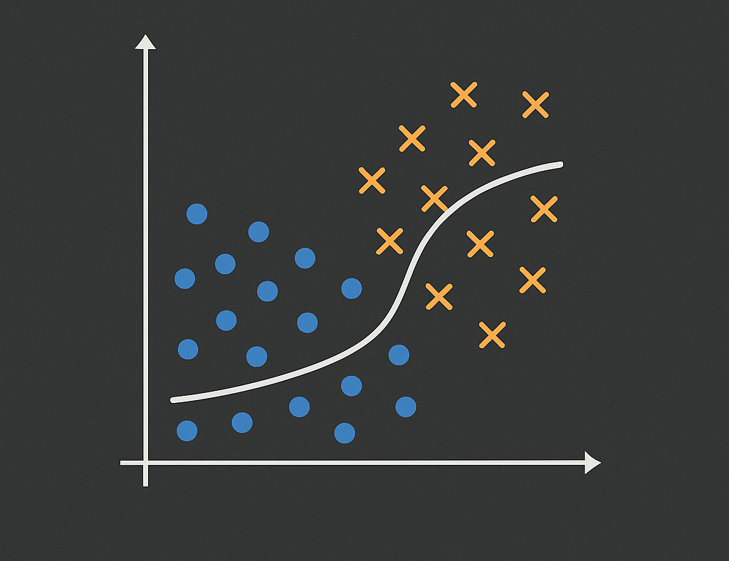
Logistic Regression (Classification)
Ce projet implémente la régression logistique à partir de zéro pour prédire la probabilité de développer une maladie cardiaque dans les 10 prochaines années, en utilisant l'ensemble de données de l'étude de Framingham Heart Study.
Vue d'ensemble du projet
Ce projet implémente la régression logistique à partir de zéro pour prédire la probabilité de développer une maladie cardiaque dans les 10 prochaines années, en utilisant l'ensemble de données de l'étude de Framingham Heart Study. Le modèle est entraîné en codant manuellement la fonction de coût (log-loss) et la descente de gradient, puis comparé avec l'implémentation de scikit-learn.
Le workflow couvre le prétraitement des données (gestion des valeurs manquantes, normalisation et ajout du biais), l'implémentation mathématique de la fonction sigmoïde, de la fonction de coût log-loss et de la descente de gradient, l'entraînement et l'évaluation du modèle, et la comparaison avec LogisticRegression de scikit-learn.
Ce projet construit une compréhension approfondie de l'algorithme de régression logistique en implémentant chaque composant mathématique à partir de zéro. Il renforce les fondements théoriques tout en démontrant des workflows pratiques de machine learning avec scikit-learn.
Fonctionnalités clés
Implémentation du code
1. Import des bibliothèques
import pandas as pd
import numpy as np
from sklearn.preprocessing import StandardScaler
from sklearn.model_selection import train_test_split
from sklearn.linear_model import LogisticRegression
from sklearn.metrics import accuracy_score, confusion_matrix, classification_report
2. Chargement et exploration du dataset
# Chargement du dataset Framingham Heart Study
df = pd.read_csv("framingham.csv")
print(df.shape)
df.head()

# Vérification des valeurs manquantes
print(df.isnull().sum())

# Nettoyage des données
df = df.drop_duplicates()
df = df.fillna(df.mean())
print("Shape after cleaning:", df.shape)
3. Fonction sigmoïde
def sigmoid(z):
    """
    Fonction sigmoïde : σ(z) = 1 / (1 + e^(-z))
    """
    return 1 / (1 + np.exp(-z))

# Test de la fonction sigmoïde
z = np.linspace(-10, 10, 100)
sigmoid_values = sigmoid(z)
4. Fonction de coût (Log Loss)
def compute_cost(X, y, theta):
    """
    Fonction de coût logistique (Log Loss)
    J(θ) = -(1/m) * Σ[y*log(h) + (1-y)*log(1-h)]
    """
    m = len(y)
    h = sigmoid(X.dot(theta))
    epsilon = 1e-5  # Pour éviter log(0)
    cost = -(1/m) * (y.dot(np.log(h+epsilon)) + (1-y).dot(np.log(1-h+epsilon)))
    return cost
5. Algorithme de descente de gradient
def gradient_descent(X, y, theta, alpha, num_iters):
    """
    Descente de gradient pour la régression logistique
    """
    m = len(y)
    cost_history = []

    for i in range(num_iters):
        # Calcul de l'hypothèse
        h = sigmoid(X.dot(theta))

        # Calcul du gradient
        gradient = (1/m) * X.T.dot(h - y)

        # Mise à jour des paramètres
        theta -= alpha * gradient

        # Sauvegarde du coût
        cost = compute_cost(X, y, theta)
        cost_history.append(cost)

        if i % 100 == 0:
            print(f"Iteration {i}: Cost={cost:.4f}")

    return theta, cost_history

# Préparation des données
X = df.drop("TenYearCHD", axis=1).values
y = df["TenYearCHD"].values

# Standardisation
scaler = StandardScaler()
X = scaler.fit_transform(X)

# Ajout du biais
X_train_bias = np.c_[np.ones(X_train.shape[0]), X_train]
X_test_bias = np.c_[np.ones(X_test.shape[0]), X_test]

# Initialisation et entraînement
theta_init = np.zeros(X_train_bias.shape[1])
theta, cost_history = gradient_descent(X_train_bias, y_train, theta_init, alpha=0.001, num_iters=100000)
6. Évaluation du modèle
# Prédictions
y_pred_prob = sigmoid(X_test_bias.dot(theta))
y_pred = (y_pred_prob >= 0.5).astype(int)

# Métriques d'évaluation
print("Accuracy:", accuracy_score(y_test, y_pred))
print("Confusion Matrix:")
print(confusion_matrix(y_test, y_pred))
print("Classification Report:")
print(classification_report(y_test, y_pred))
7. Comparaison avec scikit-learn
# Modèle scikit-learn
clf = LogisticRegression(max_iter=10000)
clf.fit(X_train, y_train)
y_pred_lib = clf.predict(X_test)

print("Sklearn Accuracy:", accuracy_score(y_test, y_pred_lib))

# Comparaison des coefficients
print("\nCoefficients comparison:")
print("Custom implementation - Final theta:", theta)
print("Sklearn - Coefficients:", clf.coef_)
print("Sklearn - Intercept:", clf.intercept_)Détails du projet
Client
Projet Personnel
Timeline
2025 – Présent
Rôle
Développeur Machine Learning
À propos du dataset
Autres projets

JobHub – Plateforme d'Emploi Intelligente avec Agent IA
Application Web Full-Stack

Email AI Platform
Intelligence Artificielle

Ovia
Intelligence Artificielle

MediBook Platform
Web Application (Healthcare SaaS)

MediBook Healthcare Passport
Web Application (Healthcare SaaS)

MediBook Pharma Platform
Web Application (Healthcare SaaS)

MediBook Laboratory Platform
Web Application (Healthcare SaaS)

Personal Portfolio Website
Web Application

Reboturn
E-Commerce Platform (Eco-Conscious SaaS)
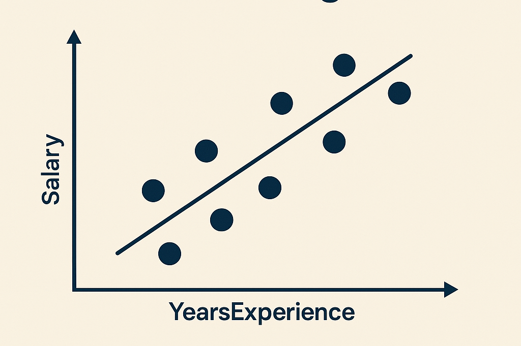
Salary Prediction with Linear Regression
Machine Learning Project

Insurance Cost Prediction with Multivariable Linear Regression
Machine Learning Project

Brain Tumor Classification (Deep Learning - CNN)
Machine Learning Project

Decision Trees
Machine Learning Project
Random Forest
Machine Learning Project
Clustering (K-means)
Machine Learning Project
Anomaly Detection
Machine Learning Project

Système de Recommandation Netflix
Intelligence Artificielle

Recommender Systems (Content-based Filtering)
Machine Learning Project

VelociType — Test de Vitesse de Frappe
Application Python

Watermark — Application de Filigrane d'Images
Application Python

XO Battle — Jeu de Tic-Tac-Toe
Jeu Python

PulseCode — Morse Converter
Application Python

DisChat – High-Performance Real-Time Chat Platform
Application Web Full-Stack
© 2026 Sina Ganji. Tous droits réservés.